Why Do We Need Analytical Models to Guide Training for Cooperative Multi-Agent Learning?
Background
Cooperative multi-agent reinforcement learning (CMARL) refers to settings in which agents share a common objective and must coordinate their actions, such as cloud scheduling and power-system operation. The training difficulty of cooperative MARL grows rapidly with the number of agents $N$, stemming from multi-agent credit assignment: when all agents jointly contribute to the shared objective, no individual agent’s contribution can be cleanly identified.
Taking QMIX as an example, all agents are trained using the same team reward, while the learning algorithm must identify each agent’s individual contribution from this shared signal, causing the noise to scale as $\Theta(N)$.

As the number of agents increases, the $\Theta(N)$-scaling noise increasingly dominates the useful gradient signal, making reliable policy updates progressively more difficult. Model-based counterfactual methods, for example, rely on accurately modeling how alternative individual actions affect system outcomes, which requires an accurate dynamics model that may be unavailable in practice and costly to obtain.
Motivation and Proposed Approach
Fortunately, many cooperative engineering systems admit differentiable analytical models that prescribe efficient system states. For example, queueing models characterize how workloads should be balanced across servers in cloud scheduling, while power-flow equations characterize how generation should meet demand subject to network constraints in power systems. These prescriptions remain system-level descriptions and do not directly yield local decision rules for individual agents.


Departing from existing approaches, we propose a new direction in which we directly use analytical models to obtain an optimal system state $\tilde{\boldsymbol{x}}=\left\lbrace\tilde{x}^n\right\rbrace_{n=1}^N$ and use this state to guide policy training. Examples include the load-balancing state in cloud scheduling, the economic-dispatch solution in power systems, and the system-optimal flow pattern in transportation networks. We only need to guide the system toward this reference state to achieve near-optimal system performance.
For example, in cloud scheduling, the optimal system state corresponds to load balance; in power systems, to optimal power flow; and in transportation networks, to system-optimal traffic flow. We only need to guide policy training so that the learned policies can more easily drive the system toward the corresponding optimal state.
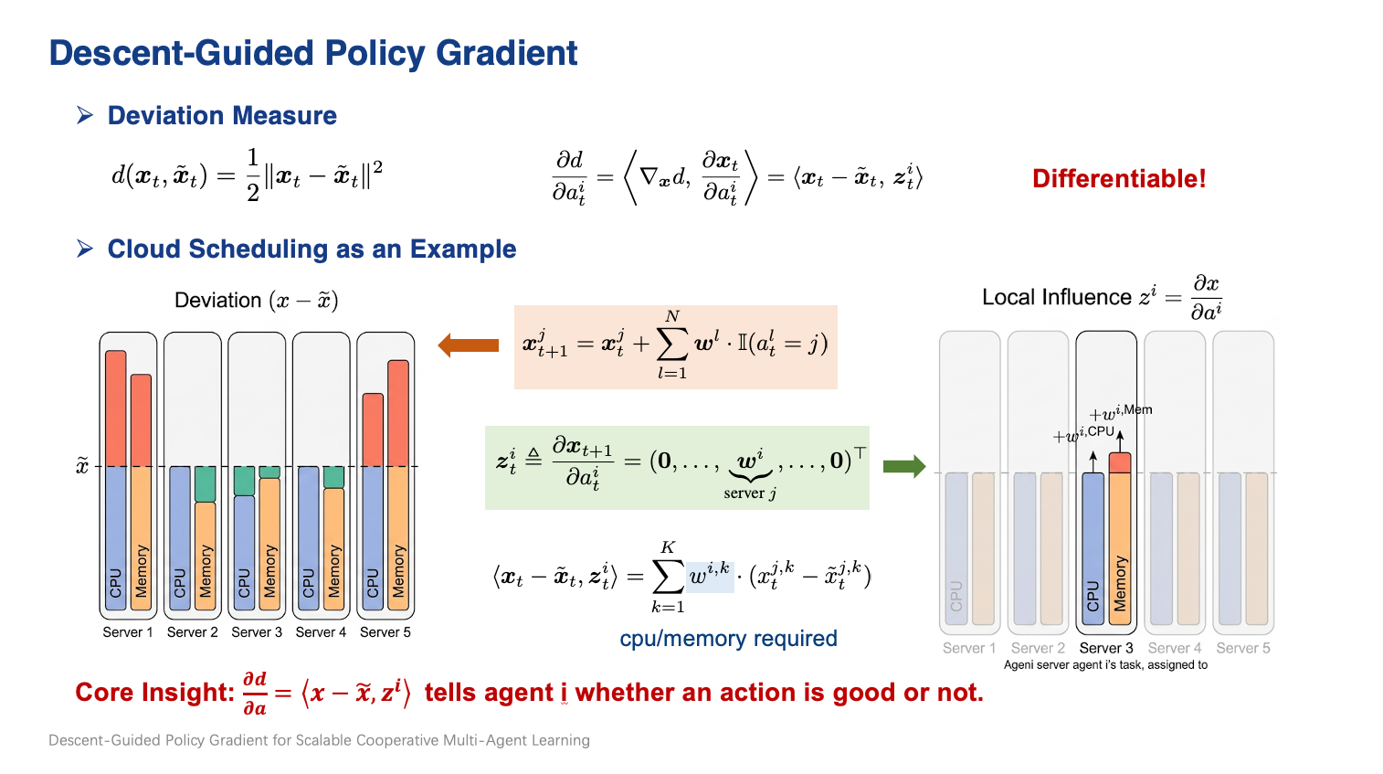
Within this system representation, each component $x_t^n$, such as the workload of a server, the power output of a generator, or the flow on a road link, is generally affected by only a limited subset of agents. This local dependence allows us to construct a low-variance guidance gradient for agent $i$ as
\[\hat{g}_{\mathcal{G},t}^i = \left\langle \boldsymbol{x}_t-\tilde{\boldsymbol{x}}_t, \boldsymbol{z}_t^i \right\rangle \nabla_{\theta^i}\log\pi^i(a_t^i\mid o_t^i),\]where $\boldsymbol{z}_t^i\triangleq\frac{\partial\boldsymbol{x}_t}{\partial a_t^i}$ represents the local influence of agent $i$ on the system state.

Taking cloud scheduling as an example, $\boldsymbol{x}_t-\tilde{\boldsymbol{x}}_t$ measures how the current workload of each server deviates from the load-balanced state, while $\boldsymbol{z}_t^i\triangleq\frac{\partial\boldsymbol{x}_t}{\partial a_t^i}$ directly indicates how agent $i$’s action changes the workload of each server. Consequently, $\hat{g}_{\mathcal G,t}^i$ identifies whether the action moves the system toward or away from load balance, providing a low-variance guidance signal for policy training.

Implementation
In implementation, DG-PG can be incorporated into any policy-gradient-based algorithm by adding one term to its original advantage. For example, in PPO, we just need to replace the original PPO advantage $\hat A_{\mathrm{PPO},t}^i$ with
\[\hat A_{\mathrm{DG},t}^i = (1-\alpha)\hat A_{\mathrm{PPO},t}^i - \alpha g_{\mathcal G,t}^i,\]where $\alpha\in[0,1]$ controls the balance between the original PPO advantage and the analytical guidance.
Computing $g_{\mathcal G,t}^i$ is also straightforward. Taking cloud scheduling as an example, suppose agent $i$ assigns a task to server $a_t^i$, where each task requires both CPU and memory. After computing the target CPU and memory utilizations $\tilde{x}_{\mathrm{CPU},t}^n$ and $\tilde{x}_{\mathrm{MEM},t}^n$ for every server $n$, the guidance term is
\[g_{\mathcal G,t}^i = \sum_{n=1}^{N} \left[ \left(x_{\mathrm{CPU},t}^n-\tilde{x}_{\mathrm{CPU},t}^n\right) z_{\mathrm{CPU},t}^{i,n} + \left(x_{\mathrm{MEM},t}^n-\tilde{x}_{\mathrm{MEM},t}^n\right) z_{\mathrm{MEM},t}^{i,n} \right],\]where $z_{\mathrm{CPU},t}^{i,n}$ and $z_{\mathrm{MEM},t}^{i,n}$ directly equal the CPU and memory demands associated with agent $i$’s action on server $n$, respectively. The resulting advantage is passed directly to the original PPO update. The critic, reward function, and all other components remain unchanged.
# analytical_state(action) returns the system state induced by this action
x = analytical_state(action)
local_influence = torch.autograd.functional.jacobian(analytical_state, action)
dgf = torch.dot(x - x_opt, local_influence)
advantage = (1 - alpha) * advantage - alpha * dgf
When the action is discrete, the local influence is directly given by the change in $\boldsymbol{x}$ caused by the selected action.
In practice, the reference state $\tilde{\boldsymbol{x}}$ does not need to satisfy the descent-alignment condition strictly. The following are some representative applications:
-
Power generation. The solution obtained from an economic dispatch problem can directly serve as the reference state $\tilde{\boldsymbol{x}}$, regardless of whether it is immediately attainable. Incorporating long-term generation dynamics may yield a better reference solution, but this is not necessary. The local influence $\boldsymbol{z}^i$ can then be obtained from the derivative of the generation state with respect to agent $i$’s generation-adjustment action.
-
Traffic information dissemination. The system-optimal traffic flow obtained from dynamic traffic assignment can be directly used as the reference state $\tilde{\boldsymbol{x}}$. The local influence $\boldsymbol{z}^i$ is then the change in traffic flow induced by agent $i$’s information-dissemination action.
-
Communication network routing. The optimal link-flow allocation obtained from a multicommodity-flow problem can be directly used as the reference state $\tilde{\boldsymbol{x}}$. The local influence $\boldsymbol{z}^i$ is then the change in link flows induced by agent $i$’s routing action.
For implementation details, see the repository below.
References
- NIPS Under Review
 Under review at NeurIPS